Modeling time-series using pytorch

This is Part 3 in the chronicles of Becky the Computational Biologist.

• Part 1 - The Computational Biologist - a short story
• Part 2 - The Side Project - a short story (regulatory network modeling)

"But cells don't operate at steady-state in reality!"

This was something Becky had heard over and over from colleagues at MidFerment Corp. They weren't wrong but that wasn't the point. After all, "All models are wrong. Some are useful," as George Box famously declared.

Usually, it was enough to simulate steady-state network flow in cellular metabolic networks. That provided enough insights into the bottlenecks that limited biomolecule production. Or, a dynamic simulation could be performed using a system of ordinary differential equations. Or even simpler, a sequence of steady-state simulations separated by small time steps.

This latest project was different. The high-throughput team had constructed hundreds of strains with different genotypes, cultured them in dozens of conditions, and had measured thousands of dynamic profiles. Growth curves, metabolite concentrations, RNA and protein. All over time. And they all looked very rich in information.

This time, the dynamics were ALL that mattered.

Not to mention that the cell factory used was a non-model organism. A mechanistic cell simulator wasn't available. And there certainly wasn't enough time to build one from scratch.

Becky had to learn everything about this cell factory's metabolism and regulation from the dynamic time profiles.

She wasn't sure yet what the best modeling approach was but reckoned The New Computational Biologist might provide some clues. She opened up the book excitedly, went to the table of contents, and located the chapter titled "Time-series modeling."

A silly program you'd never use in production

The "Time-series modeling" chapter started thusly,

This is a chapter on time-series modeling. It describes a field that was conceived, arguably, in the 1920s with the autoregressive model. WaveNet in 2016 was transformative for neural network-based time-series models, overcoming practical challenges of previous recursive neural network architectures, enabling faster and parallel training on larger data sets. Recent foundation AI models like TimeGPT have billions of parameters and hundreds of billions of timepoints across multiple domains. They can do zero-shot forecasting on unseen data without retraining, reducing development time and costs for new applications.

"Wow, that sounds amazing," thought Becky. "Also, I have no idea what that last sentence means..."

The chapter continued,

But we're going to forget all that for the moment and go back 100 years.

"Huh?" Becky thought.

Look at this code snippet, the book prompted. Do you understand what it's doing?

def time_series(t, y, k_forecast, coeffs):
    """
    Use model to forecast future based on 
    past time points (auto-regressive).
    Later, can add exogenous inputs.
    
    t: time vector
    y: response over time
    k_forecast: number of points to forecast into future
    coeffs: model coefficient vector
    """    
    # Total number of timepoints
    ny = len(y)

    # How many historical time points are used
    # for forecasting k_forecast time points?
    k_historical = ny - k_forecast

    # Get the past points
    y_historical = y[:k_historical]
    y_past = np.zeros(ny)
    y_past[:k_historical] = y_historical
    
    # Then, recursively forecast future points   
    na = len(coeffs)
    y_preds = []
    t_preds = []

    # Start from "now"
    for k in range(k_historical, ny):
        tk = t[k]
        # Get na past timepoints
        y_pastk = y_past[(k-na):(k)]
        # Weighted sum of past timepoints = future timepoint
        y_pred = sum([ci*yk for ci,yk in zip(coeffs,y_pastk)])
        # Record the forecasted response and time        
        y_preds.append(y_pred)
        t_preds.append(tk)
        
        # Update past timepoint with predicted forecast
        y_past[k] = y_pred        
            
    return t_preds, y_preds

Becky examined the code for a few minutes.

The code looked rather simple, and the comments were helpful.

Becky could tell that the code described a time-series model that could forecast future values from past ones. All implemented with a simple for loop.

"Wait," Becky thought. Using past values to predict future values. That's what an autoregressive model was!

Sure enough, the chapter explained:

The autoregressive model with exogenous inputs is:

$$
y_{k} = \sum_{i=1}^{n_a} a_i y_{k-i} + \sum_{i=1}^{n_b} b_i u_{k-i-n_k},
$$

where the autoregressive (AR) part is:

$$
y_{k} = \sum_{i=1}^{n_a} a_i y_{k-i}
$$

This AR model is coded as:

y_pred = sum([ci*yk for ci,yk in zip(coeffs,y_pastk)])

Becky was intrigured by how simple the code was. But if the code were so simple, could it reproduce any complex dynamics? Becky was doubtful.

Dynamics with one parameter

The book chapter continued,

The AR model is intuitive: we predict a future response based on past values.

The model order, or number of parameters is also intuitive. More parameters allows us to use more past time points.

What if we have only one parameter, and use only one past timepoint? We can examine four scenarios.

$y_k = a_1 y_{k-1}$

• exponential increase (unstable): $a_1 > 1$
• oscillatory increase (unstable) : $a_1 < -1$
• stable convergence to zero: $0 < a_1 < 1$
• oscillatory convergence to zero: $-1 < a_1 < 0$

The plots of each scenario is show below:

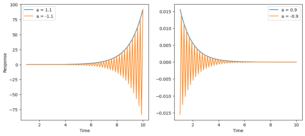
So even with one parameter, we can produce non-trivial dynamics.

Of course, we can have auto-regressive models with more parameters. And given historical data, we can learn the optimal parameter values.

"Okay, now that's a bit more surprising," Becky thought. "I wouldn't have expected such a simple code to show nonlinear and even oscillatory behavior."

Furthermore, Becky could imagine that by using more parameters len(coeffs)>1 and using more past timepoints, this simple code could potentially produce rather complex dynamics.

The question now was, how to determine the right parameter values to produce a particular dynamic profile?

Estimating model coefficients with Pytorch

As if having read Becky's mind, the chapter continued...

To estimate parameters $a_i$, we'll implement our silly code using modern AI libraries. In pytorch, you'll find the 1D convolutional neural network (CNN). Using it, we'll implement a simple time-series model.

class AR_NN(nn.Module):
    def __init__(self, na=3, out_channels=1, bias=False):
        """
        na: number of past time points of output (y) to use for prediction
        out_channels: dimension of predicted output
        """
        super().__init__()
        self.na = na
        self.layers = nn.Sequential(
            nn.Conv1d(1, out_channels, na, bias=bias)
        )
        
    def forward(self, x):
        return self.layers(x)
    
    def forecast(self, y_array, n_future):
        """
        Forecast n_future points into the future
        """
        na = self.na
        nx = len(y_array)
        
        y_all = torch.zeros((nx+n_future,1))
        y = torch.tensor(y_array)
        y_all[0:nx,0] = y
        
        with torch.no_grad():
            for k in range(n_future):
                y_prev = y_all[(nx+k-na):(nx+k)].T
                
                # Only use past points to predict future
                yp = self(y_prev)
                y_all[nx+k] = yp

        y_forecast = y_all[nx:]
        return y_forecast

Overview of the 1D CNN:

• one output channel: only predicting a univariate response
• one input channel: only past values of the response is used to predict future values
• kernel size is equal to the number of past timepoints used to predict the next value
• a single, Conv1d layer

We also add a convenient forecast method:

• uses the last $n_a$ points to predict the next time point
• to forecast the next timepoint, use past timepoints and the predicted current timepoint

this iterative approach is used to forecast values forward by any time horizon.

Becky inspected this new code. It wasn't much more complicated than the "silly" manual code from before. In fact, it seemed like the the AR formulation was encoded into one line:

self.layers = nn.Sequential(nn.Conv1d(1, out_channels, na, bias=bias)

Also, the forecast method seemed similar to what the manual code was doing: taking na past timepoints to predict the next timepoint.

Suddenly, Becky came to a realization. Since this was just a neural network written using Pytorch, she could use the package's built-in optimization methods to estimate the model coefficients.

She wrote up a simple training routine using mean-squared error minimization between known and predicted time profiels as the objective. She then set up the Adam optimizer, with a learning rate of 0.001.

"What about the training data," Becky thought.

She decided that instead of using all the real growth curves, she'd prototype the program using synthetic data created from a known function.

The logistic growth curve seemed like a good choice. For a population abundance $p$ with growth rate $\mu$, the logistic model was

$$
\frac{dp}{dt} = \mu (1-p) p.
$$

It had an exponential growth region and a plateauing stationary phase. She wrote up the logistic model, set random growth rates and generated 50 growth profiles.

She then arranged the data into time windows, providing windows of timepoints na = 3 time steps into the past, and for each window providing the next timepoint value as the prediction. She now had a training data set.

Excited, Becky set up training batches, ran the Adam optimizer and, to her satisfaction, saw the loss values drop rapidly over 100 epochs of training.

Forecasting

The model had been trained, and coefficients estimated. All that was left was to try forecasting value and seeing if the model was accurate.

Then, Becky had an idea.

Since the 1D CNN had estimated 3 coefficients for an AR(3) model, the same coefficients should also work for the manual "silly" program she'd written earlier.

She extracted the coefficients from the Conv1d layer, and provided them as the coefficients to the manual AR code. She then used the forecasting function to plot 50 timepoints into the future, at timepoint 50.

She got the following plot:

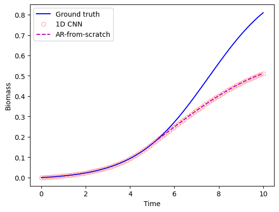
"Yes!" Becky exclaimed. The 1D CNN coded up in pytorch and the autoregressive model she'd written up from scratch produced identical results.

Becky knew that in the grand scheme of things, this was a tiny victory. After all, all she'd done was created an autoregressive model two different ways and confirmed they yielded the same result.

But strangely enough, this exercise of training a time-series model from two directions: from scratch, and using a neural network via pytorch, gave here a strange sense of confidence.

In undergrad, she felt she'd understood the equations for time-series models. And using Matlab functions, she could certainly train models using a variety of lab data.

But she'd never written an AR model from scratch. Nor had she thought she could write one using a 1D CNN.

Furthermore, Becky realized that she already knew what to do next. Exogenous inputs.

The New Computational Biologist had described ARX, auto-regressive with exogenous inputs. This meant that Becky could take other measurements besides the growth curve itself to make predictions. She knew the high-throughput team had measured media component concentration dynamics for a smaller number of experiments. And in all cases, there was meta data about the experimental conditions.

Becky knew that she could extend her simple 1D CNN in several ways:

• more input channels to account for more inputs
• larger kernel size (larger $n_a$) to capture more complex dynamics
• add more layers to account for even more complex dynamics

She also noted the book mentioned using "dilation." She saw that this was analogous to larger time steps, or less frequent sampling. In other words, with the same number of model parameters, by skipping timesteps, she could use data points further into the past to forecast the future. The book showed modified code to implement dilation but Becky was confident she understood the model well enough that she could implement it herself.

Closing

Becky was excited. In a short time, she'd acquired a deeper understanding of basic time-series modeling. She also knew on a fundamental level what time-series model using neural networks entailed.

This meant she had great freedom to extend the sophistication of her model, and apply it to larger data sets. The parallel architecture of 1D CNN would allow her to train large time-series data efficiently on the GPU.

Becky opened the spreadsheet of 5,000 growth curves that her colleagues had sent her on Monday.

This time, she looked at the dizzying array of numbers, not with apprehension but with a calm curiosity.

"I wonder how simple my model can get while reproducing all these dynamics?" she thought. And what causality could she identify between exogenous inputs and the outputs? This was going to be a fun project.

Enjoyed the story? Curious about The Computational Biologist book that helped Becky cut through complexity and leverage simplicity?

Join the newsletter

Get access to exclusive chapter previews, computational biology insights, and be first to know when the full book launches.